Pairwise Image Registration#
This tutorial is an introduction to using the deepali library for the spatial alignment of two images.
Let’s begin with the common imports used throughout this tutorial.
import os
from typing import Any, Callable, Optional, Tuple, Type, cast

from IPython.utils import io
from matplotlib.figure import Figure
import matplotlib.pyplot as plt
from tqdm.notebook import tqdm

import torch
from torch import Tensor, optim
try:
    from deepali.core.environ import cuda_visible_devices
except ImportError:
    if not os.getenv("COLAB_RELEASE_TAG"):
        raise
    !git clone https://github.com/BioMedIA/deepali.git && pip install ./deepali
    from deepali.core.environ import cuda_visible_devices
Choose CUDA device to use if available. By default, this tutorial runs on the CPU.
os.environ["CUDA_VISIBLE_DEVICES"] = "0"

# Use first device specified in CUDA_VISIBLE_DEVICES if CUDA is available
device = torch.device("cuda:0" if torch.cuda.is_available() and cuda_visible_devices() else "cpu")
Dataset#
The images used in this tutorial are from the public MNIST dataset available through torchvision.
from torchvision.datasets import MNIST
from torchvision.transforms import ToTensor

with io.capture_output() as captured:  # type: ignore[reportPrivateImportUsage]
    mnist = MNIST(root="data", download=True, transform=ToTensor())
Next we define a utility function named imshow for displaying the example images used in this tutorial.
def imshow(
    image: Tensor,
    label: Optional[str] = None,
    ax: Optional[plt.Axes] = None,
    **kwargs,
) -> None:
    r"""Render image data in last two tensor dimensions using matplotlib.pyplot.imshow().

    Args:
        image: Image tensor of shape ``(..., H, W)``.
        ax: Figure axes to render the image in. If ``None``, a new figure is created.
        label: Image label to display in the axes title.
        kwargs: Keyword arguments to pass on to ``matplotlib.pyplot.imshow()``.
            When ``ax`` is ``None``, can contain ``figsize`` to specify the size of
            the figure created for displaying the image.

    """
    if ax is None:
        figsize = kwargs.pop("figsize", (4, 4))
        _, ax = plt.subplots(figsize=figsize)
    kwargs["cmap"] = kwargs.get("cmap", "gray")
    ax.imshow(image.reshape((-1,) + image.shape[-2:])[0].cpu().numpy(), **kwargs)
    if label:
        ax.set_title(label, fontsize=16, y=1.04)
    ax.get_xaxis().set_visible(False)
    ax.get_yaxis().set_visible(False)
We can now display a random selection of the MNIST dataset to select an example pair of images to register.
digits = tuple(range(10))

n_rows = len(digits)
n_cols = 10

rng = torch.Generator().manual_seed(0)
perm = torch.randperm(len(mnist), generator=rng)

samples: dict[int, list[Tensor]] = {digit: [] for digit in digits}
for i in perm:
    image, digit = mnist[i]
    samples[digit].append(image)
    if all(len(samples[digit]) >= n_cols for digit in digits):
        break
samples = {digit: images[:n_cols] for digit, images in samples.items()}

_, axes = plt.subplots(n_rows, n_cols, figsize=(n_cols, n_rows), tight_layout=True)
for row, digit in zip(axes, digits):
    for ax, image in zip(row, samples[digit]):
        imshow(image, ax=ax)
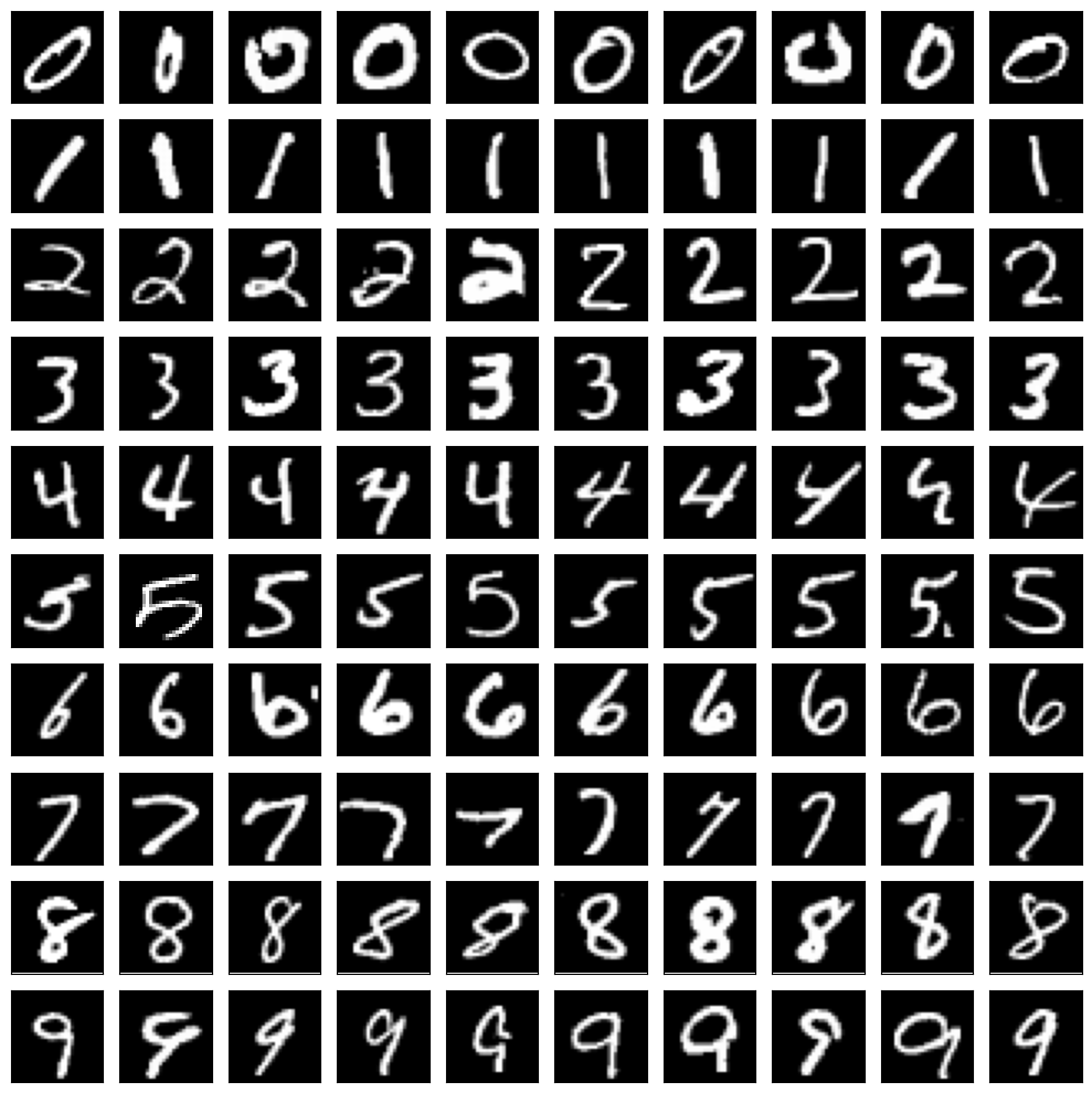
target = samples[9][0].float()
source = samples[9][2].float()

_, axes = plt.subplots(1, 2, figsize=(8, 4), tight_layout=True)

imshow(target, "target", ax=axes[0])
imshow(source, "source", ax=axes[1])
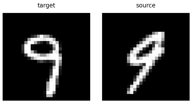
Let’s now try and align the source image of our chosen digit with the target image.
First, we define a spatial transformation model which determines the type of spatial transformation that we want to apply. As we have chosen two examples with a different rotation, we select an EulerRotation from the deepali.spatial library. This transformation has a single parameter in 2D, namely the rotation angle. Each spatial transformation is defined with respect to normalized coordinates as used by torch.nn.functional.grid_sample(). Every spatial transform with base type SpatialTransform maps points given with respect to these coordinates to normalized coordinates defined with respect to the same domain, i.e., the domain and codomain of the normalized coordinate map is the same. As these normalized coordinates range are in [-1, 1] for the extent of each image side, the origin of this coordinate system is in the image center. The rotation is thus also with respect to the image center.
For images sampled on a regular grid, we use the Grid class defined by deepali.core to convert between different coordinate systems. An instance of Grid is also used by the spatial transform to define its domain and codomain, respectively. Commonly, this is the sampling grid of the fixed target image, though it need not be. It could also be a subimage region or a reference space if both images were symmetrically mapped to this common space. For medical images, the Grid defines the mapping between image element indices, world coordinates, and the normalized coordinates. The position of the image within the world is defined by the Grid.center() (or Grid.origin()), its orientation by the Grid.direction() cosines matrix, and the extent of each image element in world units by Grid.spacing() (e.g., millimeters).
In case of MNIST, we simply use a world coordinate system which is identical to the image space.
from deepali.core import Grid

grid = Grid(shape=target.shape[1:])

print("size:     ", list(grid.size()))
print("origin:   ", grid.origin().tolist())
print("center:   ", grid.center().tolist())
print("spacing:  ", grid.spacing().tolist())
print("direction:", grid.direction().tolist())
size:      [28, 28]
origin:    [-13.5, -13.5]
center:    [0.0, 0.0]
spacing:   [1.0, 1.0]
direction: [[1.0, 0.0], [0.0, 1.0]]
Images in world space
The objective of image registration is traditionally with respect to their alignment within the world coordinate system. This is especially important when aligning images from different sources or with point clouds (e.g., from depth sensors). In deep learning applications, the alignment is often carried out with respect to the normalized coordinates and the image to world map is ignored. However, when exporting a spatial transform for visualization or to use with classic registration tools such as ANTs, ITK, MIRTK, NiftyReg and others, we need to recover the correct world information and also convert the spatial transform to a world coordinate map. For this purpose, the Grid and more specifically FlowField tensor type of the deepali.data library will come in handy, though we will cover this in another tutorial.
Grid center vs. origin
Notice that grid stores the position of the image center as attribute, from which the image origin, i.e., the world coordinates of the sampling point with all zero indices, is computed using the grid spacing and direction. This simplifies grid resizing operations, including increasing (e.g., Grid.upsample()) and decreasing (e.g., Grid.downsample()) the number of image sampling points along each spatial grid dimension. We will go into more details on the different coordinate systems and relation between them in a separate tutorial when working with medical image volumes.
Grid size vs. shape
The Grid properties are defined with respect to world coordinate axes in the order x, y, etc. The Grid.shape property, however, is in reverse order to match the ordering of the spatial dimensions in the corresponding image data tensor which has shape (C, ..., Y, X), where C is the number of image channels, and ..., Y, X is the size of the image and thus sampling grid along the respective spatial dimension. The Grid.size() and size argument of the Grid init function specify the size of each spatial dimension in the original order, i.e., x, y, etc. The torch.Tensor.size() uses the ordering of Grid.shape. In order to not confuse the different ordering of spatial dimensions, it is adviced to prefer torch.Tensor.shape over torch.Tensor.size(), which is also consistent with the use of numpy.ndarray.shape and Grid.shape.
Grid search#
To begin, let’s try a brute force grid search of the optimal angle which minimizes a chosen objective. The objective used measures the similarity of the fixed target and moving source images as proxy for assessing the quality of the spatial alignment. For the grid search, we manually set the rotation angle to different values, evaluate our chosen similarity measure, and keep a record of the current optimal angle which thus far attained the minimum value.
Similarity or loss?
Though in image registration we often refer to the data fidelty term of the objective function as similarity measure, by convention the value reflects a dissimilarity or spatial alignment error rather which we want to minimize. A similarity measure which increases in value with better spatial alignment of the images may be negated to minimize this function. Furthermore, to align with the terminology used in deep learning, all objective function terms are named losses and thereby defined in the deepali.losses library.
Here, we select the mean squared error (MSE) as our similarity measure.
from deepali.losses import functional as L

sim_loss = L.mse_loss
Spatial transformation modules are defined by the deepali.spatial library.
import deepali.spatial as spatial
With a normalized coordinate map given in the form of a SpatialTranform, we need an operation which applies this spatial transformation to the moving source image. There are different functions in deepali which can be used for this, which are all built on torch.nn.functional.grid_sample(). These are mainly the grid_sample() function of the functional deepali.core API, the image sampling modules defined in deepali.modules, and the spatial transformer modules defined in deepali.spatial. The latter can be directly combined with a spatial transform without having to work with the normalized coordinates explicitly. Unlike a SpatialTransform, a SpatialTransformer takes as input a tensor representing the data to which the spatial transformation should be applied. The ImageTransformer more specifically takes as input an image batch tensor of shape (N, C, ..., Y, X) and samples it at the spatially transformed grid points of the fixed target image domain.
target_batch = target.unsqueeze(0)  # (N, C, Y, X)
source_batch = source.unsqueeze(0)  # (N, C, Y, X)

rotation = spatial.EulerRotation(grid, params=False)
transformer = spatial.ImageTransformer(rotation)

angle_space = torch.linspace(-180.0, 180.0, 360)
best_angle_deg = torch.tensor(0.0)
min_loss_value = torch.tensor(torch.inf)

bar_format = "{l_bar}{bar}{rate_fmt}{postfix}"
for angle_deg in (pbar := tqdm(angle_space, bar_format=bar_format)):
    rotation.angles_(angle_deg.deg2rad().reshape(1, 1))
    warped_batch = transformer(source_batch)
    loss = sim_loss(warped_batch, target_batch)
    if loss.lt(min_loss_value):
        best_angle_deg = angle_deg
        min_loss_value = loss
        pbar.set_postfix(dict(loss=loss.item(), angle=angle_deg.item()))

rotation.angles_(best_angle_deg.deg2rad().reshape(1, 1))
warped: Tensor = transformer(source_batch)[0]

fig, axes = plt.subplots(1, 3, figsize=(12, 4), tight_layout=True)

imshow(target, "target", ax=axes[0])
imshow(warped, "warped", ax=axes[1])
imshow(source, "source", ax=axes[2])
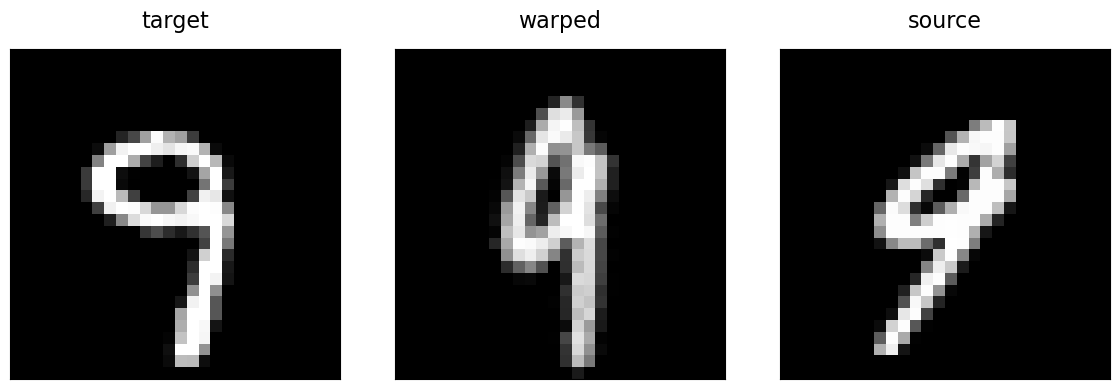
For the grid search, we used params=False in the init function of the spatial transform to indicate that the parameters of the transform (the Euler angle in case of the chosen 2D rotation) are non-optimizable. With this setting, the SpatialTransform.parameters() function of the torch.nn.Module subclass returns an iterator over an empty collection and the params property of the spatial transform is of type torch.Tensor. With the default setting of params=True, the params property is of type torch.nn.parameter.Parameter instead. We will use it in the next section.
Gradient descent#
While for this toy example with a single parameter, grid search is a viable option, the number of objective function evalutions grows exponentially with the number of parameters of our spatial transform, and moreover grid search requires a discretization of our parameter space. We can use the gradient descent optimization normally used in PyTorch in fitting a neural network to a training set also to perform a gradient descent to optimize the image alignment.
target_batch = target.unsqueeze(0)  # (N, C, Y, X)
source_batch = source.unsqueeze(0)  # (N, C, Y, X)

rotation = spatial.EulerRotation(grid)
transformer = spatial.ImageTransformer(rotation)
optimizer = optim.Adam(transformer.parameters(), lr=1e-2)

iterations = 100

bar_format = "{l_bar}{bar}{rate_fmt}{postfix}"
for _ in (pbar := tqdm(range(iterations), bar_format=bar_format)):
    warped_batch = transformer(source_batch)
    loss = sim_loss(warped_batch, target_batch)
    angle_deg = rotation.angles().rad2deg().item()
    pbar.set_postfix(dict(loss=loss.item(), angle=angle_deg))
    optimizer.zero_grad()
    loss.backward()
    optimizer.step()

with torch.inference_mode():
    warped: Tensor = transformer(source_batch)[0]

fig, axes = plt.subplots(1, 3, figsize=(12, 4), tight_layout=True)

imshow(target, "target", ax=axes[0])
imshow(warped, "warped", ax=axes[1])
imshow(source, "source", ax=axes[2])
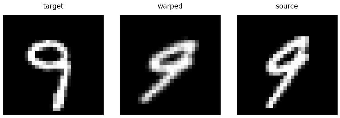
Unfortunately, for this given pair of images and the chosen optimizer and hyperparameters such as learning rate and momentum, the registration resulted in a suboptimal solution compared to our previous grid search result. What happened?
Gradient descent is a local optimization technique and sensitive to the initialization. Furthermore, the binary nature of the images with a lot of homogeneous regions (background mostly) and the chosen similarity measure result in an insufficient signal (capture range) from our objective in which way to adjust our rotation at each gradient step in order to minimize the loss and thereby maximize alignment. Increasing and decreasing the angle by a little bit changes our objective value similarly, so it is difficult to judge which is the better direction to follow.
Multi-scale registration#
The way this is overcome in traditional optimization based image registration is via a multi-scale or multi-resolution optimization scheme, respectively. For this, we first downsample the images a number of times, find the optimal rotation between those lower resolution images with a wider spatial extent of each image element, and continue with the next higher resolution with the solution found at the lower resolution. To generate a multi-scale representation of our images, Gaussian blurring is commonly applied. This is also to obey the Nyquist-Shannon sampling theorem when subsampling the image signal. The resulting pyramid of differently sized images is referred to as Gaussian image pyramid. In deep learning based image registration, a multi-scale representation of the input images is usually obtained by the employed neural network.
Sampling grid pyramid
Notice that the Grid.pyramid() function can be used to construct the sampling grids for the different scales of the image pyramid. The corresponding function of the Image tensor type of the deepali.data library generates both, the data tensors of the different pyramid scales and assigns the respective sampling grid with the images at each scale.
Multi-scale vs. multi-resolution
Note that multi-scale optimization in case of a rigid transformation such as a rotation would already by achieved by simply using a multi-scale representation of the images by blurring the images with consecutively larger Gaussian kernels (or consecutively with the same kernel) without also reducing the image size itself. In non-rigid registration, the images downsampled mainly for two reasons: a) to reduce the resolution of the image deformation field, and b) to reduce the computational cost at lower scales. In deepali.spatial the non-rigid transformations such as DisplacementFieldTransform and FreeFormDeformation have a stride parameter which can be used to reduce the size of the non-rigid transformation without changing the image sampling grid. Here, we are using a standard multi-resolution image pyramid with downsampling.
from deepali.data import Image

levels = 3

target_pyramid = Image(target, grid).pyramid(levels)
source_pyramid = Image(source, grid).pyramid(levels)

fig, axes = plt.subplots(2, levels, figsize=(4 * levels, 8), tight_layout=True)

for (level, tgt), src in zip(target_pyramid.items(), source_pyramid.values()):
    imshow(tgt, f"target, level {level}", ax=axes[0, level])
    imshow(src, f"source, level {level}", ax=axes[1, level])
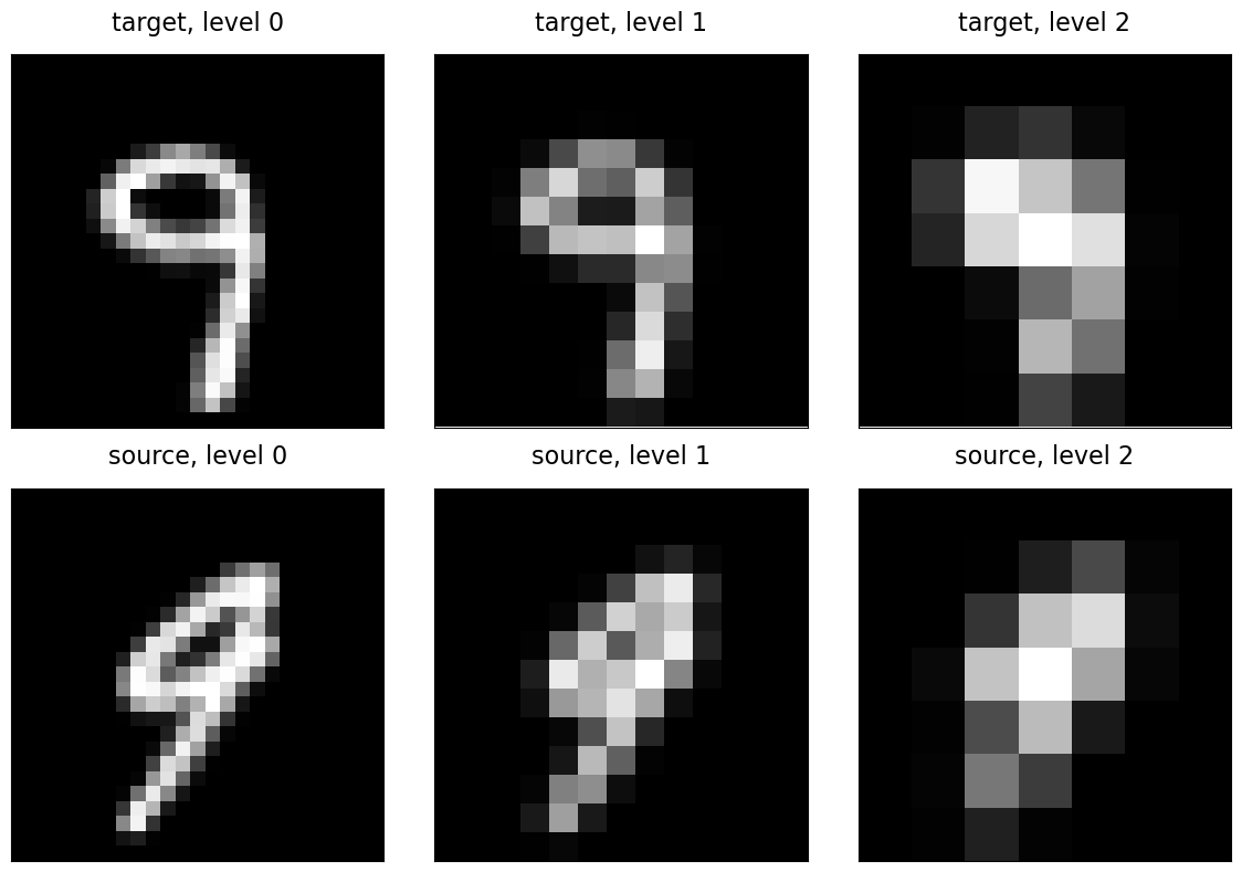
With these image pyramids, we can implement a sequential multi-resolution registration as follows.
ImagePyramid = dict[int, Image]
LossFunction = Callable[[Tensor, Tensor, spatial.SpatialTransform], Tensor | dict[str, Tensor]]
TransformCls = str | Type[spatial.SpatialTransform]
TransformArg = TransformCls | Tuple[TransformCls, dict[str, Any]]
OptimizerCls = str | Type[optim.Optimizer]
OptimizerArg = OptimizerCls | Tuple[OptimizerCls, dict[str, Any]]


def image_pyramid(
    image: Tensor | Image | ImagePyramid,
    levels: int,
    grid: Optional[Grid] = None,
    device: Optional[torch.device] = None,
) -> ImagePyramid:
    r"""Consruct image pyramid from image tensor."""
    if isinstance(image, dict):
        pyramid = {}
        for level, im in image.items():
            if type(level) is not int:
                raise TypeError("Image pyramid key values must be int")
            if level >= levels:
                break
            if type(im) is Tensor:
                im = Image(im, grid)
            if not isinstance(im, Image):
                raise TypeError("Image pyramid key values must be deepali.data.Image or torch.Tensor")
            im = cast(Image, im.float().to(device))
            pyramid[level] = im
        if len(pyramid) < levels:
            raise ValueError(f"Expected image pyramid with {levels} levels, but only got {len(pyramid)} levels")
    else:
        if not isinstance(image, Image):
            image = Image(image, grid)
        image = cast(Image, image.float().to(device))
        pyramid = image.pyramid(levels)
    return pyramid


def init_transform(transform: TransformArg, grid: Grid, device: Optional[torch.device] = None) -> spatial.SpatialTransform:
    r"""Auxiliary functiont to create spatial transform."""
    if isinstance(transform, tuple):
        cls, args = transform
    else:
        cls = transform
        args = {}
    if isinstance(cls, str):
        spatial_transform = spatial.new_spatial_transform(cls, grid, **args)
    else:
        spatial_transform = cls(grid, **args)
    return spatial_transform.to(device).train()


def init_optimizer(optimizer: OptimizerArg, transform: spatial.SpatialTransform) -> optim.Optimizer:
    r"""Auxiliary function to initialize optimizer."""
    if isinstance(optimizer, tuple):
        cls, args = optimizer
    else:
        cls = optimizer
        args = {}
    if isinstance(cls, str):
        cls = getattr(optim, cls)
    if not issubclass(cls, optim.Optimizer):
        raise TypeError("'optimizer' must be a torch.optim.Optimizer")
    return cls(transform.parameters(), **args)


def multi_resolution_registration(
    target: Tensor | Image | ImagePyramid,
    source: Tensor | Image | ImagePyramid,
    loss_fn: LossFunction,
    transform: TransformArg,
    optimizer: OptimizerArg,
    iterations: int | list[int] = 100,
    levels: int = 3,
    device: Optional[str | int | torch.device] = None,
) -> spatial.SpatialTransform:
    r"""Multi-resolution pairwise image registration."""
    if device is None:
        if isinstance(target, dict):
            device = next(iter(target.values())).device
        else:
            device = target.device
    device = torch.device(f"cuda:{device}" if type(device) is int else device)
    target = image_pyramid(target, levels=levels, device=device)
    levels = len(target)
    source = image_pyramid(source, levels=levels, device=device)
    model = init_transform(transform, target[levels - 1].grid(), device=device)
    bar_format = "{l_bar}{bar}{rate_fmt}{postfix}"
    if isinstance(iterations, int):
        iterations = [iterations]
    iterations = list(iterations)
    iterations += [iterations[-1]] * (levels - len(iterations))
    for level, steps in zip(reversed(range(levels)), iterations):
        model.grid_(target[level].grid())
        target_batch = target[level].batch().tensor()
        source_batch = source[level].batch().tensor()
        transformer = spatial.ImageTransformer(model)
        optim = init_optimizer(optimizer, model)
        for _ in (pbar := tqdm(range(steps), bar_format=bar_format)):
            warped_batch: Tensor = transformer(source_batch)
            loss = loss_fn(warped_batch, target_batch, model)
            if isinstance(loss, Tensor):
                loss = dict(loss=loss)
            pbar.set_description(f"Level {level}")
            pbar.set_postfix({k: v.item() for k, v in loss.items()})
            optim.zero_grad()
            loss["loss"].backward()
            optim.step()
    return model.eval()
Let’s see what we now obtain for the rigid registration of our two digits using this registration function:
transform = multi_resolution_registration(
    target=target,
    source=source,
    transform=spatial.EulerRotation,
    optimizer=(optim.Adam, {"lr": 1e-2}),
    loss_fn=lambda a, b, _: sim_loss(a, b),
    device=device,
)
transform = transform.cpu()

with torch.inference_mode():
    transformer = spatial.ImageTransformer(transform)
    warped: Tensor = transformer(source)

fig, axes = plt.subplots(1, 3, figsize=(12, 4), tight_layout=True)

imshow(target, "target", ax=axes[0])
imshow(warped, "warped", ax=axes[1])
imshow(source, "source", ax=axes[2])
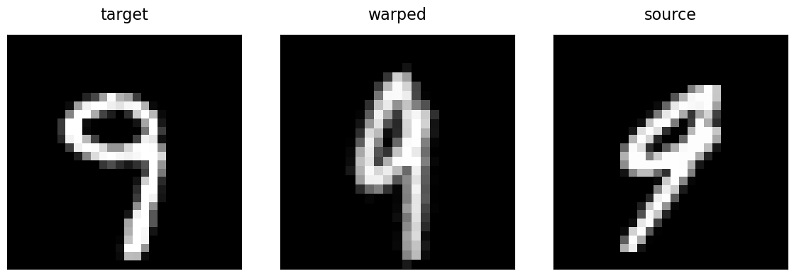
Great! The multi-resolution gradient descent resulted in a similar solution as the previous exhaustive grid search.
Non-rigid registration#
Multi-resolution optimization becomes even more important when the spatial transform is non-rigid. Apart from linearly interpolated dense vector fields, a free-form deformation based on a cubic B-spline parameterization is commonly employed in medical image registration. This non-rigid transformation model has the advantage that first and second order derivatives can be computed exactly. Using our previously defined multi_resolution_registration() function, we can alternatively optimize a non-rigid deformation such as a spatial.FreeFormDeformation (FFD).
def loss_fn(
    w_curvature: float = 0,
    w_diffusion: float = 0,
    w_bending: float = 0,
) -> Callable[[Tensor, Tensor, spatial.SpatialTransform], dict[str, Tensor]]:
    r"""Construct loss function for free-form deformation (FFD) based image registration.

    Args:
        w_curvature: Weight of curvature, i.e., sum of unmixed first order derivatives.
            When the spatial transform is parameterized by velocities, the curvature of
            the velocity vector field is computed.
        w_bending: Weight of bending energy, i.e., sum of second order derivatives.

    Returns:
        Loss function which takes as input a registered image pair, and the spatial transform
        used to register the images. The loss function evaluates the alignment of the images
        based on a similarity term and optional regularization terms (transform penalties).

    """

    def loss(
        warped: Tensor,
        target: Tensor,
        transform: spatial.SpatialTransform,
    ) -> dict[str, Tensor]:
        terms: dict[str, Tensor] = {}
        # Similarity term
        sim = sim_loss(warped, target)
        terms["sim"] = sim
        loss = sim
        # Regularization terms
        # v_or_u: dense velocity or displacement vector field, respectively.
        v_or_u = getattr(transform, "v", getattr(transform, "u", None))
        assert v_or_u is not None
        if w_curvature > 0:
            curvature = L.curvature_loss(v_or_u)
            loss = curvature.mul(w_curvature).add(loss)
            terms["curv"] = curvature
        if w_diffusion > 0:
            diffusion = L.diffusion_loss(v_or_u)
            loss = diffusion.mul(w_diffusion).add(loss)
            terms["diff"] = diffusion
        if w_bending > 0:
            if isinstance(transform, spatial.BSplineTransform):
                params = transform.params
                assert isinstance(params, Tensor)
                bending = L.bspline_bending_loss(params)
            else:
                bending = L.bending_loss(v_or_u)
            loss = bending.mul(w_bending).add(loss)
            terms["be"] = bending
        return {"loss": loss, **terms}

    return loss
transform = multi_resolution_registration(
    target=target_pyramid,
    source=source_pyramid,
    transform=("FFD", {"stride": 2}),
    optimizer=("Adam", {"lr": 1e-2}),
    loss_fn=loss_fn(w_bending=1e-5),
    device=device,
)
transform = transform.cpu()

with torch.inference_mode():
    transformer = spatial.ImageTransformer(transform)
    warped: Tensor = transformer(source)

fig, axes = plt.subplots(1, 3, figsize=(12, 4), tight_layout=True)

imshow(target, "target", ax=axes[0])
imshow(warped, "warped", ax=axes[1])
imshow(source, "source", ax=axes[2])
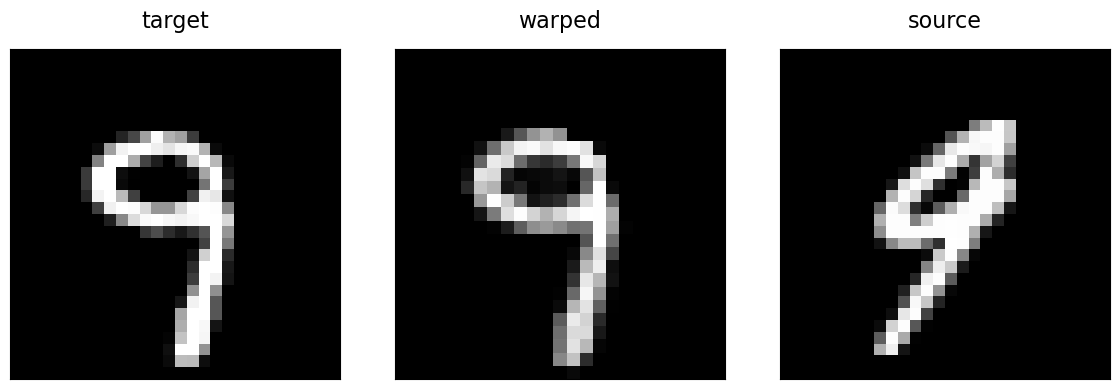
In addition to the choice of parameterization of the spatial transform (i.e., vector field given by a cubic B-spline with control points at every second image grid point), we added a loss term (bspline_bending_loss()) which penalizes bending of the spline. By setting the weight of this term w_bending to higher values, we can make the spatial transform stiffer and allow for less severe deformation. In order to assess the quality of the computed deformation, we can visualize the deformation of the image grid. Because of the small size of the MNIST images, we generate a higher resolution grid image for this visualization, which we then deform using an ImageTransformer with an input source and output target grid matching this higher resolution.
from deepali.core import functional as U


grid_highres = grid.resize(512)
grid_image = U.grid_image(grid_highres, num=1, stride=8, inverted=True)
grid_transformer = spatial.ImageTransformer(transform, grid_highres, padding="zeros")

with torch.inference_mode():
    warped_grid: Tensor = grid_transformer(grid_image)

fig, axes = plt.subplots(1, 2, figsize=(8, 4), tight_layout=True)

imshow(grid_image, "source grid", ax=axes[0])
imshow(warped_grid, "warped grid", ax=axes[1])
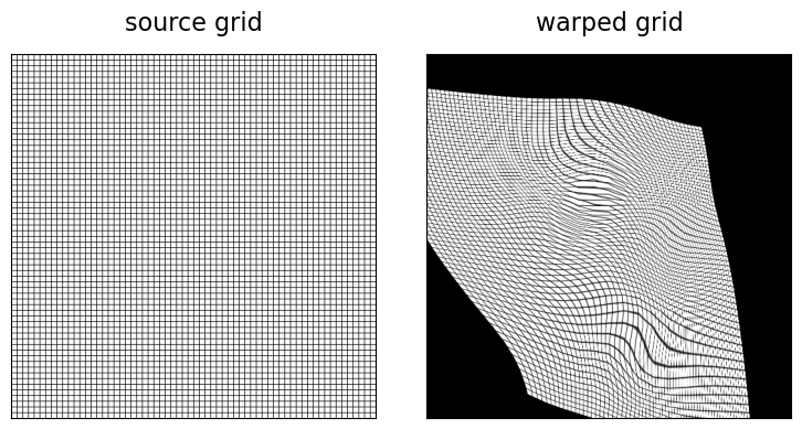
Although the deformed source image matches well our target image, we realize that our deformation is not well behaved. This can be remedied by increasing the weight of the bending loss (w_bending).
transform = multi_resolution_registration(
    target=target_pyramid,
    source=source_pyramid,
    transform=(spatial.FreeFormDeformation, {"stride": 2}),
    optimizer=(optim.Adam, {"lr": 1e-2}),
    loss_fn=loss_fn(w_bending=1e-3),
    device=device,
)
transform = transform.cpu()

with torch.inference_mode():
    image_transformer = spatial.ImageTransformer(transform)
    grid_transformer = spatial.ImageTransformer(transform, grid_highres, padding="zeros")
    warped_grid: Tensor = grid_transformer(grid_image)
    warped: Tensor = image_transformer(source)

fig, axes = plt.subplots(1, 4, figsize=(16, 4), tight_layout=True)

imshow(target, "target", ax=axes[0])
imshow(warped, "warped", ax=axes[1])
imshow(source, "source", ax=axes[2])
imshow(warped_grid, "deformation", ax=axes[3])

Diffeomorphic registration#
In the previous non-rigid registration example, we used a free form deformation model as our spatial transformation. Though with a good choice of the control point spacing (stride) and bending regularization weight (w_bending) we ended up with a smooth and invertible spatial transform, sometimes it is desireable to have the property of being able to invert a spatial transform with both the forward and backward map being differentiable, baked into the chosen transformation model. Typically, a diffeomorphic coordinate map is parameterized either by a time-varying or stationary velocity vector field (SVF). The latter is more commonly found in the recent registration literature because of its computational efficiency. We can use the scaling and squaring algorithm to compute the exponential map of this vector field to compute the dense displacement field generated by this velocity field.
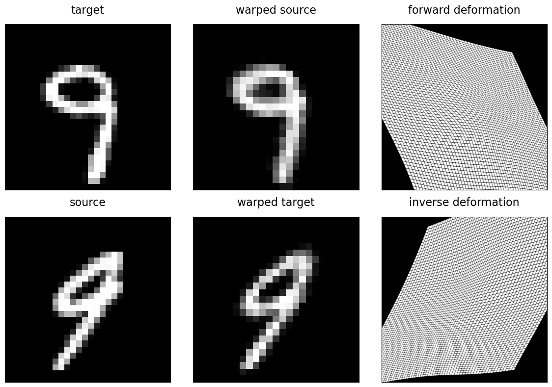
The spatial.StationaryVelocityFieldTransform (SVF) and spatial.StationaryVelocityFreeFormDeformation (SVFFD) are diffeomorphic transformation models based on such stationary velocity field. We can use the SpatialTransform.inverse() funtion to obtain the inverse deformation. With this, we can define the following auxiliary function to plot the result of a diffeomorphic registration, where the source image is deformed by the computed forward transform and the target image is deformed with its inverse, respectively.
def invertible_registration_figure(
    target: Tensor,
    source: Tensor,
    transform: spatial.SpatialTransform,
) -> Figure:
    r"""Create figure visualizing result of diffeomorphic registration.

    Args:
        target: Fixed target image.
        source: Moving source image.
        transform: Invertible spatial transform, i.e., must implement ``SpatialTransform.inverse()``.

    Returns:
        Instance of ``matplotlib.pyplot.Figure``.

    """
    device = transform.device

    highres_grid = transform.grid().resize(512)
    grid_image = U.grid_image(highres_grid, num=1, stride=8, inverted=True, device=device)

    with torch.inference_mode():
        inverse = transform.inverse()

        source_transformer = spatial.ImageTransformer(transform)
        target_transformer = spatial.ImageTransformer(inverse)

        source_grid_transformer = spatial.ImageTransformer(transform, highres_grid, padding="zeros")
        target_grid_transformer = spatial.ImageTransformer(inverse, highres_grid, padding="zeros")

        warped_source: Tensor = source_transformer(source.to(device))
        warped_target: Tensor = target_transformer(target.to(device))

        warped_source_grid: Tensor = source_grid_transformer(grid_image)
        warped_target_grid: Tensor = target_grid_transformer(grid_image)

    fig, axes = plt.subplots(2, 3, figsize=(12, 8), tight_layout=True)

    imshow(target, "target", ax=axes[0, 0])
    imshow(warped_source, "warped source", ax=axes[0, 1])
    imshow(warped_source_grid, "forward deformation", ax=axes[0, 2])

    imshow(source, "source", ax=axes[1, 0])
    imshow(warped_target, "warped target", ax=axes[1, 1])
    imshow(warped_target_grid, "inverse deformation", ax=axes[1, 2])

    return fig
We use the previously implemented multi_resolution_registration helper to optimize a diffeomorphic transformation. Here, we selected the SVFFD with a control point at every other image grid point. Note that the stride is in number of grid points. This way, the resolution of the control point grid is defined by the resolution of the target image at the current level of the mult-resolution optimization.
transform = multi_resolution_registration(
    target=target_pyramid,
    source=source_pyramid,
    transform=(spatial.StationaryVelocityFreeFormDeformation, {"stride": 2}),
    optimizer=(optim.Adam, {"lr": 1e-2}),
    loss_fn=loss_fn(w_bending=1e-3),
    device=device,
)
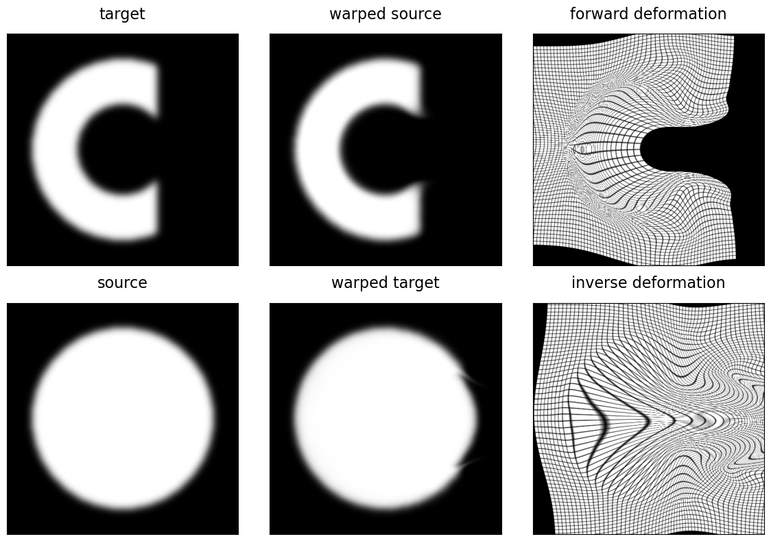
The visualization shows both good alignment between the deformed source image and target, as well as good alignment between the target deformed by the inverse and the input source image.
_ = invertible_registration_figure(target, source, transform)
Circle to C deformation#
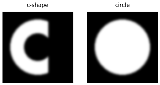
A classic example for demonstrating a diffeomorphic registration is the “circle to C” problem, where an image of a circle is deformed to align it with the image of the letter “C”. This example has been used in the DARTEL paper by John Ashburner, one of the seminal works which first introduced this parameterization for use in medical image registration. We can generate a similar example, though at present with a more open and thus more challenging target “C” shape, using functions cshape_image() and circle_image() of the deepali.core library. Gaussian blurring is applied to smooth the edges of these synthetic binary images.
fig, axes = plt.subplots(1, 2, figsize=(8, 4))

circle_c_grid = Grid((128, 128))
target_cshape = U.cshape_image(circle_c_grid, radius=50, sigma=2, dtype=torch.float)
source_circle = U.circle_image(circle_c_grid, radius=50, sigma=2, dtype=torch.float)

imshow(target_cshape, "c-shape", ax=axes[0])
imshow(source_circle, "circle", ax=axes[1])
circle_to_c_transform = multi_resolution_registration(
    target=target_cshape[0],
    source=source_circle[0],
    loss_fn=loss_fn(w_diffusion=1e-3),
    transform=spatial.StationaryVelocityFreeFormDeformation,
    optimizer=(optim.Adam, {"lr": 1e-2}),
    iterations=[200, 200, 300, 100],
    levels=4,
    device=device,
)
_ = invertible_registration_figure(target_cshape, source_circle, circle_to_c_transform)
